
1.1 Problem description
Assume a scenario in which fluid is enclosed between two coaxial cylinders that can be considered infinitely long from a mathematical point of view. In practice, however, these usually have a finite length. This mathematical approximation makes it possible to model the two-dimensional case without first taking into account the influences of the boundary conditions.
The fluid under consideration is incompressible and Newtonian, and the flow is assumed to be laminar. The cylinders each rotate at an individual angular velocity Ω1 or Ω2. The radii of the cylinders are designatedR1 andR2, with the Z-axis representing the coaxial cylinder axis.
In the literature, the resulting fluid movement is known as Couette flow, a special form of flow between rotating cylinders. The investigation of this phenomenon provides insights into the complex flow conditions and is of interest for a wide range of applications in the fields of fluid mechanics, engineering and physics.
1.2 Analytical solution
The analytical solution is based on the solution of the Navier-Stokes equations for incompressible fluids. It proves advantageous to consider the geometry at hand using cylindrical coordinates, which simplifies the calculations and exploits the symmetry of the problem.
The symmetry shows that the axial velocity (uz) and the radial velocity (ur) of the fluid are both zero,
while the circumferential speed is considered as a function of the radius r. Similarly, the pressure p varies as a function of the radius r
These correlations facilitate the analytical calculation of the Navier-Stokes equations and thus form the basis for the development of solutions to the flow problem between the cylinders.
In the same way that the speed of a solid body can be calculated by solving Newton’s second law,
the velocity of a fluid (liquid or gas) can be calculated by solving the Navier-Stokes equations.
The Navier-Stokes equations are analogous to Newton’s second law and state that the rate of change of momentum of a fluid is equal to the sum of the external forces acting on the fluid. However, the Navier-Stokes equations are applied to a finite volume of fluid rather than a solid body.
The following general notation of the equations can often be found in the literature:
- Radial momentum equation:r:ρ(∂ur∂t+ur∂ur∂r+uφr∂ur∂φ−u2φr+uz∂ur∂z)=−∂p∂r+μ(1r∂∂r(r∂ur∂r)+1r2∂2ur∂φ2+∂2ur∂z2−urr2−2r2∂uφ∂φ)+13μ(1r∂∂r(rur)+1r∂uφ∂φ+∂uz∂z)+ρgr
- Axial momentum equation: φ:ρ(∂uφ∂t+ur∂uφ∂r+uφr∂uφ∂φ+uz∂uφ∂z−uruφr)=−1r∂p∂φ+μ(1r∂∂r(r∂uφ∂r)+1r2∂2uφ∂φ2+∂2uφ∂z2−uφr2−2r2∂ur∂φ)+13μr(1r∂∂r(rur)+1r∂uφ∂φ+∂uz∂z)+ρgφ
- Azimuthal momentum equation: z:ρ(∂uz∂t+ur∂uz∂r+uφr∂uz∂φ+uz∂uz∂z)=−∂p∂z+μ(1r∂∂r(r∂uz∂r)+1r2∂2uz∂φ2+∂2uz∂z2)+13μ(1r∂∂r(rur)+1r∂uφ∂φ+∂uz∂z)+ρgz
Equations (1) and (2) can be solved decoupled from each other. The second has the solution of type
The constants a and b can be obtained from the boundary conditions on cylinder surfaces. The fluid adheres to these due to the so-called “no slip” condition and therefore has the same velocities as the cylinders themselves:
Inserting the constants gives the velocity distribution over the circumference:
To obtain the pressure distribution in the fluid, equation (3) is used in (1):
The solution to this differential equation can be determined by separating the variables:
All the unknowns we are looking for have now been determined and we can examine a concrete example with numerical values.
1.3 Concrete example
- R1 = 70 mm,
- R2 = 100 mm
- Ω1 = 180 RPM ≈ 18.85 rad/s
- Ω2 = -Ω1
- ρ = 970 kg/m3 (density at room temperature)
- η = 0.0216019 kg/m/s (we need the dynamic viscosity later for the numerics)
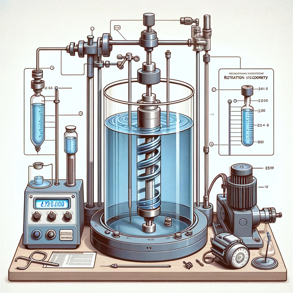
1.4 Numerical model
Three calculations with different discretizations are performed:
- fine and structured mesh,
- medium-coarse and structured mesh,
- coarse and unstructured network. Only the “default” settings were adopted by the program.
1.5 Analytics vs. numerics
We dedicate ourselves to analyzing the system. In the current task, we are interested in the velocity field of the fluid and the associated pressure distribution. Additional issues such as temperature distribution or critical rotational velocities can also be considered. Depending on the analysis, these are significantly more complex and must be treated separately.
Before the solution can be found, the expectations of the system must be considered. There are two cylinders rotating in opposite directions with adherent fluid on the surfaces. It is therefore expected that the fluid velocities on these surfaces correspond to the tangential velocities of the cylinders, i.e. uφ,i=RiΩi, i=[1,2]. As the cylinders rotate in opposite directions, there will be a change of direction in the velocity distribution.
1.5.1 Speed
Equation (3) analytically describes the velocity field of the fluid. After inserting the values, the field can be represented graphically. Since we are not only interested in the analytical closed-form solution, but also in the numerical approximate solution, we have these represented in different mesh qualities. For a better representation of the results, the velocity field is not formed in its individual components, but as a magnitude. Although this eliminates any information about the velocity direction at first glance, it turns out to be useful in the later representation.
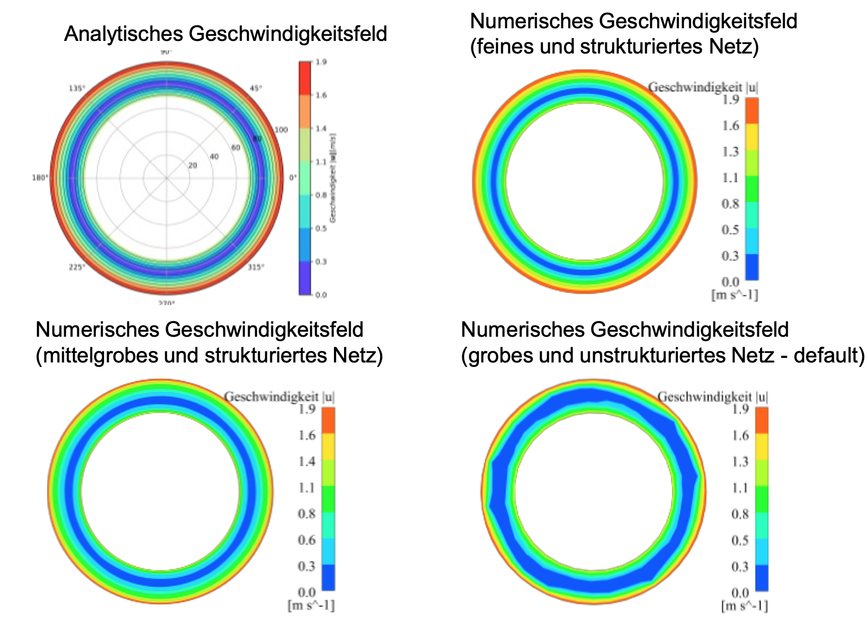
The analytical solution shows different velocities from zero at the surfaces of the cylinders and a range in between where the velocity actually assumes the value zero. This is where the change in direction of the velocity occurs. The expectations are therefore fulfilled.
At first superficial glance, the images differ only slightly from each other. What can be recognized without effort is that the results with the “default” mesh are merely less accurate, but by and large reflect the analytics. Unfortunately, the numerically generated “colored images” alone are not always meaningful and numerical values are needed at this point to make a serious comparison between analytics and numerics. In order to analyze the results in more detail, a path is laid through the fluid that represents the physical properties in the fluid. The L2 norm of the velocity over the radius (from the start of the path at R1 to the end of the path at R2) is displayed graphically:

As expected, the tangential velocities of the fluid at the beginning and end of the plot should correspond to the tangential velocities of the cylinders at R1 and R2:
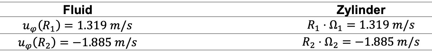
Our expectations have been fully met.
If we now turn to the numerical results of the CFD analysis, we can see more clearly how large the simulation errors are with poor meshes. Only the good and structured mesh reproduces the analytical results of the calculation with sufficient accuracy.
1.5.2 Pressure
As with the velocity distribution, the velocity field is now determined. Equation (4) analytically describes the corresponding pressure distribution in the fluid. The distributions are shown graphically below.
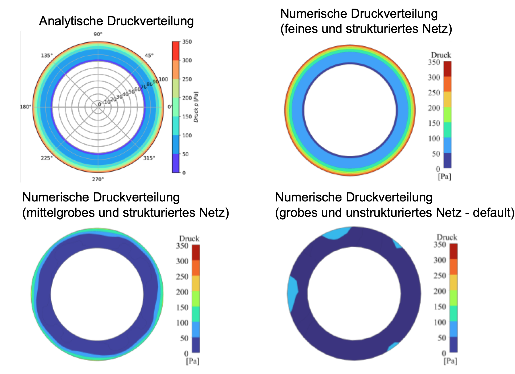
The deviation of the numerics from the analytics can also be clearly seen in these figures. The influence of the mesh is much greater than with the velocity field.
Here too, the pressure is evaluated via the same path as in the speed:

Here too, the network quality plays an enormously important role in the results and the error with poor networks is greater than can be seen in the speed field.
1.6 Conclusion
Even with supposedly simple problems, it is surprisingly easy to fall into the trap of errors and inaccuracies and the resulting calculations can be of dubious quality. The validation of numerical models is therefore of crucial importance. Without solid validation, whether through analytical methods or experimental data, there is a risk of producing worthless or incorrect results.
Modern Computational Fluid Dynamics (CFD) programs in particular often suggest an almost effortless solution to flow problems. With their “default” settings, they relieve the user of a considerable amount of work. However, there is a potential danger here: although the generated result is quickly available, it is not necessarily correct. The simulation results often deviate considerably from reality.
This phenomenon is particularly evident in the present simple studies in a two-dimensional space with incompressible, stationary and laminar flow conditions. Although the numerical solution appears acceptable at first glance, errors can occur even under seemingly trivial conditions, which severely affect the result. This emphasizes the need to carefully validate numerical models and understand the limitations of their applicability.
If you do not consider yourself an experienced user of numerics or if the analytical methods seem too complicated and abstract to you, it is advisable to turn to specialists. These specialists have the necessary know-how and experience to solve complex problems from industry and research and achieve accurate results.